Getting Started

Contents

• Getting Started
• Contents
• Installation and usage
• Model data
• Geographic and population data
• Epidemic parameters
• Initialization of the epidemics
• Containment strategy
• Running the model

Installation and usage

Installation:

] add MMCAcovid19

Usage:

using MMCAcovid19

Model data

The execution of the model depends on the following input data:

• Geographic and population data.
• Epidemic parameters.
• Initialization of the epidemics.
• Containment strategy.

For a good simulation, you need to find real data or appropriate estimates for all of them. We suppose all this information can be read from external sources, feeding the corresponding Julia variables. In what follows, we first initialize all the necessary data, sometimes using random values, to show the correct way to introduce them to our model, and finally we show how to run the model.

Geographic and population data

Here we create random geographic and population data just to show the list and structure of the data variables.

We set first the basic sizes of the system, the number of patches and the number of strata:

# Number of strata
G = 3

# Number of patches
M = 5

Now we generate a random population, i.e., the number of people at each strata and patch. We distribute a total population of one million people using a multinomial random number:

# Random population
using Random
using Distributions

g_probs = [0.1, 0.6, 0.3]
m_probs = [0.05, 0.10, 0.15, 0.30, 0.40]
probs = transpose(m_probs) .* g_probs
total_population = 1000000
distrib = Multinomial(total_population, reshape(probs, (1, G * M))[1, :])
nᵢᵍ = convert.(Float64, reshape(rand(distrib), (G, M)))

Total population: 1000000
Matrix nᵢᵍ:
  1:    4995.0    9875.0   14970.0   30010.0   40326.0
  2:   30107.0   59630.0   90009.0  179745.0  239983.0
  3:   15145.0   29827.0   45086.0   90266.0  120026.0

Note that, for convenience, we have used Float64 instead of integers to hold the sizes of the population. Now, the matrix of probabilities of contacts between strata, with all rows summing to one:

# Strata contacts
C = [0.5980 0.3849 0.0171
     0.2440 0.7210 0.0350
     0.1919 0.5705 0.2376]

For the generation of the random mobility matrix, we first create a random directed network between patches, add self-loops to each node to represent people for which work and residence patches coincide, assign random weights to all the edges, and normalize the output weights to represent the commuting probabilities. The result is a two-column matrix edgelist with the origins and destinations of each edge, and a vector R with the corresponding commuting probabilities:

# Random mobility
using LightGraphs

# network
network = erdos_renyi(M, 0.7, is_directed=true)
for i in 1:M
  add_edge!(network, i, i)   # add self-loops
end
# list of edges
L = ne(network)
edgelist = zeros(Int64, L, 2)
edgelist[:, 1] .= src.(edges(network))
edgelist[:, 2] .= dst.(edges(network))
# list of commuting probabilities
Rᵢⱼ = rand(L)
sum_r = zeros(M)
for e in 1:L   # find output strengths
  i = edgelist[e, 1]
  sum_r[i] += Rᵢⱼ[e]
end
for e in 1:L   # normalize weights
  i = edgelist[e, 1]
  Rᵢⱼ[e] /= sum_r[i]
end

Mobility matrix R:
  1 -> 1 : 0.128441
  1 -> 2 : 0.421710
  1 -> 3 : 0.065699
  1 -> 4 : 0.057292
  1 -> 5 : 0.326857
  2 -> 1 : 0.218382
  2 -> 2 : 0.407707
  2 -> 5 : 0.373911
  3 -> 1 : 0.128047
  3 -> 2 : 0.219577
  3 -> 3 : 0.190232
  3 -> 4 : 0.289372
  3 -> 5 : 0.172772
  4 -> 1 : 0.367028
  4 -> 2 : 0.295921
  4 -> 3 : 0.294488
  4 -> 4 : 0.026881
  4 -> 5 : 0.015681
  5 -> 3 : 0.379312
  5 -> 4 : 0.145112
  5 -> 5 : 0.475577

Finally, the rest of the variables related to population:

# Average number of contacts per strata
kᵍ = [11.8, 13.3, 6.6]

# Average number of contacts at home per strata
kᵍ_h = [3.15, 3.17, 3.28]

# Average number of contacts at work per strata
kᵍ_w = [1.72, 5.18, 0.0]

# Degree of mobility per strata
pᵍ = [0.0, 1.0, 0.05]

# Patch surfaces (in km²)
sᵢ = [10.6, 23.0, 26.6, 5.7, 61.6]

# Density factor
ξ = 0.01

# Average household size
σ = 2.5

Now, we are in condition to create the data structure to hold all the parameters related with the geographic area and its population:

population = Population_Params(G, M, nᵢᵍ, kᵍ, kᵍ_h, kᵍ_w, C, pᵍ, edgelist, Rᵢⱼ, sᵢ, ξ, σ)

Epidemic parameters

The epidemic parameters control the probabilities of transition between the different compartments, and are summarized in the model diagram:

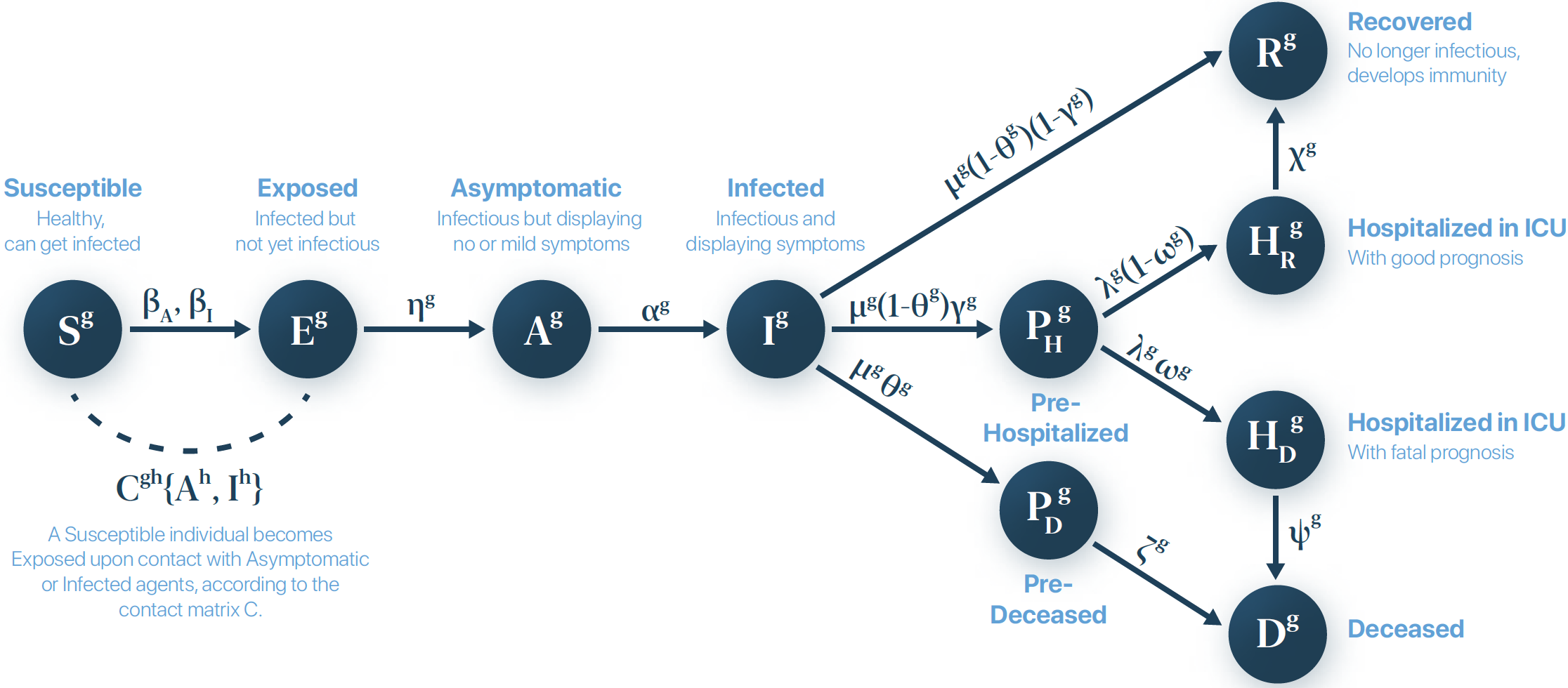
Thus, we must set them all according to the reported values in the scientific literature. Here we set the values in reference [1] of References:

# Infectivity of infected
βᴵ = 0.075

# Infectivity of asymptomatic
βᴬ = 0.5 * βᴵ

# Exposed rate
ηᵍ = [1/2.444, 1/2.444, 1/2.444]

# Asymptomatic infectious rate
αᵍ = [1/5.671, 1/2.756, 1/2.756]

# Infectious rate
μᵍ = [1/1.0, 1/3.915, 1/3.915]

# Direct death probability
θᵍ = [0.0, 0.008, 0.047]

# ICU probability
γᵍ = [0.0003, 0.003, 0.026]

# Pre-deceased rate
ζᵍ = [1/7.084, 1/7.084, 1/7.084]

# Pre-hospitalized in ICU rate
λᵍ = [1/4.084, 1/4.084, 1/4.084]

# Fatality probability in ICU
ωᵍ = [0.3, 0.3, 0.3]

# Death rate in iCU
ψᵍ = [1/7.0, 1/7.0, 1/7.0]

# ICU discharge rate
χᵍ = [1/20.0, 1/20.0, 1/20.0]

Additionally, we must set the number of timesteps (equivalent to days) to run the model equations:

# Number of timesteps
T = 200

With them, we create the corresponding data structure:

# Epidemic parameters
epi_params = Epidemic_Params(βᴵ, βᴬ, ηᵍ, αᵍ, μᵍ, θᵍ, γᵍ, ζᵍ, λᵍ, ωᵍ, ψᵍ, χᵍ, G, M, T)

Initialization of the epidemics

The initialization of the epidemic spreading is performed by introducing the initial number of infected individuals (exposed, asymptomatic and symptomatic) at each patch and strata.

# Initial number of exposed individuals
E₀ = zeros(G, M)

# Initial number of infectious asymptomatic individuals
A₀ = zeros(G, M)
A₀[2, 5] = 2.0
A₀[3, 3] = 1.0

# Initial number of infectious symptomatic individuals
I₀ = zeros(G, M)
I₀[2, 5] = 1.0

Initial number of exposed E₀:
  1:  0.0  0.0  0.0  0.0  0.0
  2:  0.0  0.0  0.0  0.0  0.0
  3:  0.0  0.0  0.0  0.0  0.0
Initial number of infectious asymptomatic A₀:
  1:  0.0  0.0  0.0  0.0  0.0
  2:  0.0  0.0  0.0  0.0  2.0
  3:  0.0  0.0  1.0  0.0  0.0
Initial number of infectious symptomatic I₀:
  1:  0.0  0.0  0.0  0.0  0.0
  2:  0.0  0.0  0.0  0.0  1.0
  3:  0.0  0.0  0.0  0.0  0.0

Now we apply the initialization:

set_initial_infected!(epi_params, population, E₀, A₀, I₀)

Containment strategy

The containment strategy relies on the timestep at which the containment is applied, the mobility reduction, the permeablity of confined households, and the social distancing:

# Timestep of application of containment
tᶜ = 30

# Mobility reduction
κ₀ = 0.65

# Permeability of confined households
ϕ = 0.174

# Social distancing
δ = 0.207

To apply multiple containments at different timesteps, just put them in lists:

# List of timesteps of application of containments
tᶜs = [30, 60, 90, 120]

# List of mobility reductions
κ₀s = [0.65, 0.75, 0.65, 0.55]

# List of permeabilities of confined households
ϕs = [0.174, 0.174, 0.174, 0.174]

# List of social distancings
δs = [0.207, 0.207, 0.207, 0.207]

Running the model

Let us summarize first the preparation of the data to feed the model:

using MMCAcovid19

# Geographic and population data
population = Population_Params(G, M, nᵢᵍ, kᵍ, kᵍ_h, kᵍ_w, C, pᵍ, edgelist, Rᵢⱼ, sᵢ, ξ, σ)

# Epidemic parameters
epi_params = Epidemic_Params(βᴵ, βᴬ, ηᵍ, αᵍ, μᵍ, θᵍ, γᵍ, ζᵍ, λᵍ, ωᵍ, ψᵍ, χᵍ, G, M, T)

# Initialization of infectious people
set_initial_infected!(epi_params, population, E₀, A₀, I₀)

With this information we can run the model:

# Run the model
run_epidemic_spreading_mmca!(epi_params, population; verbose = true)

To include a containment strategy, just add the corresponding parameters:

# Run the model with a single containment strategy
run_epidemic_spreading_mmca!(epi_params, population; tᶜ = tᶜ, κ₀ = κ₀, ϕ = ϕ, δ = δ)

Otherwise, if multiple containment strategies are needed:

# Run the model with a single containment strategy
run_epidemic_spreading_mmca!(epi_params, population, tᶜs, κ₀s, ϕs, δs; verbose = false)

The results can be stored to files using:

# Output path and suffix for results files
output_path = "output/folder"
suffix = "run01"

# Store compartments
store_compartment(epi_params, population, "S", suffix, output_path)
store_compartment(epi_params, population, "E", suffix, output_path)
store_compartment(epi_params, population, "A", suffix, output_path)
store_compartment(epi_params, population, "I", suffix, output_path)
store_compartment(epi_params, population, "PH", suffix, output_path)
store_compartment(epi_params, population, "PD", suffix, output_path)
store_compartment(epi_params, population, "HR", suffix, output_path)
store_compartment(epi_params, population, "HD", suffix, output_path)
store_compartment(epi_params, population, "R", suffix, output_path)
store_compartment(epi_params, population, "D", suffix, output_path)

If you are interested in the evolution of the effective reproduction number R for each strata and patch, or the total one, you can calculate or store them to file:

# Optional kernel length
τ = 21

# Calculate effective reproduction number R
Rᵢᵍ_eff, R_eff = compute_R_eff(epi_params, population, τ)

# Calculate and store effective reproduction number R
store_R_eff(epi_params, population, suffix, output_path, τ)